#matplotlib入门
##x轴和y轴
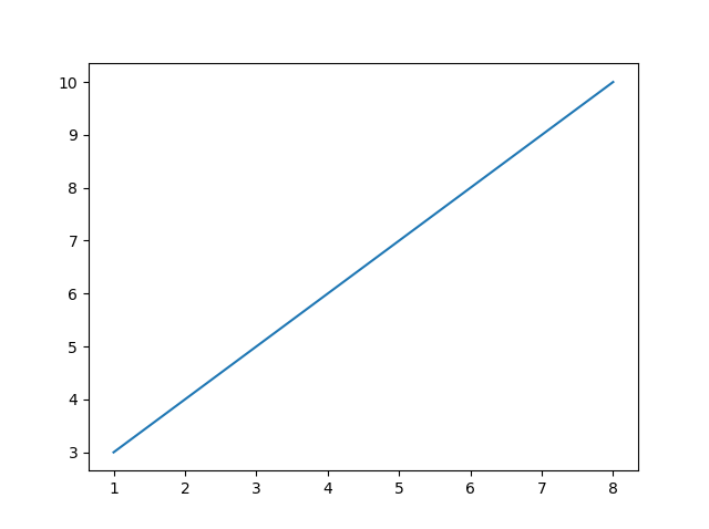
matplotlib比较难写,我们一般缩写成plt。用plot()方法进行绘制图像,第一个参数表示x轴,第二个参数表示y轴
xpoints = np.array([1, 8])
ypoints = np.array([3, 10])
plt.plot(xpoints, ypoints)
plt.show()
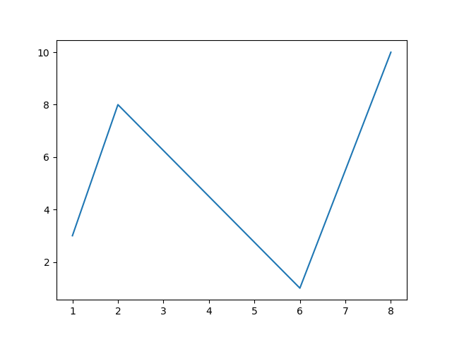
画多个点(有连线)
xpoints = np.array([1, 2, 6, 8])
ypoints = np.array([3, 8, 1, 10])
plt.plot(xpoints, ypoints)
plt.show()
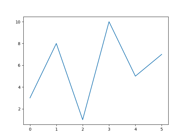
tips:这里的x轴是有默认值的,如果你没有传入x轴的参数,默认是从0开始增长,到传入y轴的参数个数-1
ypoints = np.array([3, 8, 1, 10, 5, 7])
plt.plot(ypoints)
plt.show()
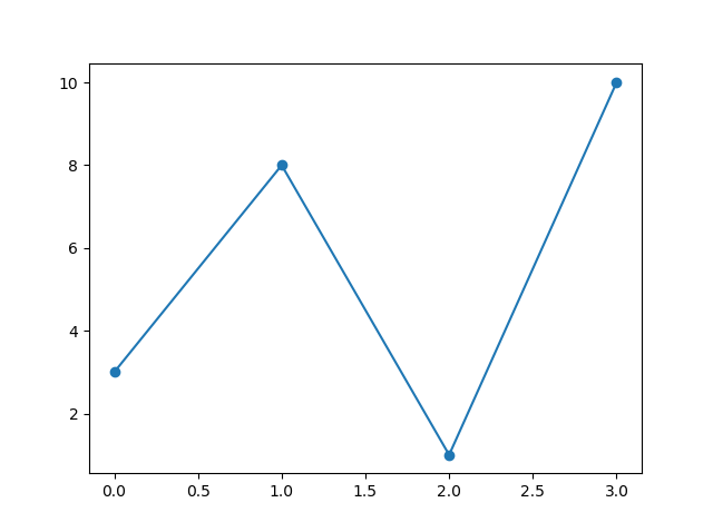
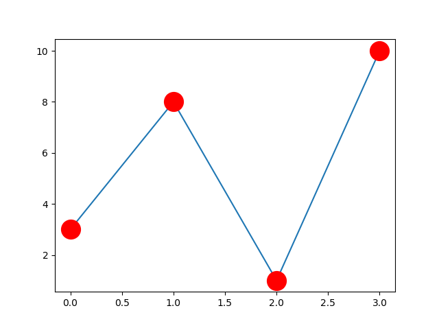
参数marker
marker用指定的标记来强调每个点
marker=’o’,对应的坐标会变成实心小圆点
ypoints = np.array([3, 8, 1, 10])
plt.plot(ypoints, marker = 'o')
plt.show()
| marker | 图像 |
|---|---|
| ‘o’ | 实心原点 |
| ‘*’ | * |
| ‘.’ | .(小点) |
| ‘,’ | 像素(我看不到) |
| ‘x’ | X |
| ‘X’ | X (粗的) |
| ‘+’ | + |
| ‘P’ | +(粗的) |
| ‘s’ | 实心正方形 |
| ‘D’ | 斜方棱形 |
| ‘d’ | 斜棱形(窄一点) |
| ‘p’ | 五边形 |
| ‘H’ | 六边形(平的) |
| ‘h’ | 六边形(竖着的,尖朝上) |
| ‘v’ | 倒三角 |
| ‘^’ | 正三角 |
| <’ | 三角(尖朝左) |
| ‘>’ | 三角(尖朝右) |
| ‘1’ | |
| ‘2’ | |
| ‘3’ | |
| ‘4’ | |
| ‘ | ’ |
| ‘_’ | _ |
格式字符串fmt
也可以使用快捷字符串符号参数来指定标记。
该参数也被称为fmt,并使用以下语法编写:
*marker*|*line*|*color*
| 线 | 形状 |
|---|---|
| ‘-‘ | 实线 |
| ‘:’ | 点虚线 |
| ‘–’ | 线虚线 |
| ‘-.’ | 点线交错虚线 |
如果不指定颜色,默认是蓝色
如果不指定线的形状,就没有线
如果不指明点的形状,就没有点
| 颜色对应字符 | 颜色 |
|---|---|
| ‘r’ | 红色 |
| ‘g’ | 绿色 |
| ‘b’ | 蓝色 |
| ‘c’ | 青色(Cyan) |
| ‘m’ | 洋红色(Magenta) |
| ‘y’ | 黄色 |
| ‘k’ | 黑色 |
| ‘w’ | 白色 |
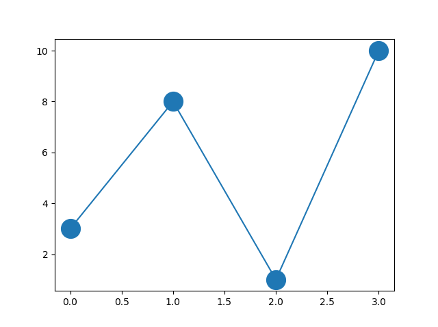
marksize
指定点的大小,参数为marksize,或者缩写成ms
ypoints = np.array([3, 8, 1, 10])
plt.plot(ypoints, marker = 'o', ms = 20)
plt.show()
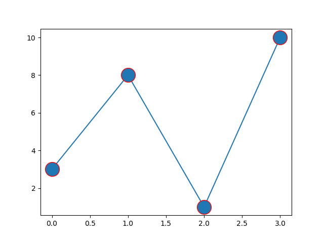
markeredgecolor
markeredgecolor设置点的边缘的颜色,可以缩写成mec
ypoints = np.array([3, 8, 1, 10])
plt.plot(ypoints, marker = 'o', ms = 20, mec = 'r')
plt.show()
markerfacecolor
markerfacecolor设置点的里面的颜色,可以缩写成mfc
ypoints = np.array([3, 8, 1, 10])
plt.plot(ypoints, marker = 'o', ms = 20, mfc = 'r')
plt.show()
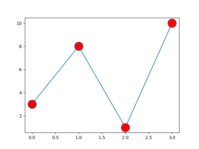
ypoints = np.array([3, 8, 1, 10])
plt.plot(ypoints, marker = 'o', ms = 20, mec = 'r', mfc = 'r')
plt.show()
这个mec和mfc可以用十六进制表示颜色,也可以用一些颜色的名字指定
plt.plot(ypoints, marker = 'o', ms = 20, mec = '#4CAF50', mfc = '#4CAF50')
plt.plot(ypoints, marker = 'o', ms = 20, mec = 'hotpink', mfc = 'hotpink')
linestyle
linestyle指定线的格式,实际上用的最多的还是上面的fmt(方便),缩写成ls
| 形状 | 参数 |
|---|---|
| ‘solid’ (default) | ‘-‘ |
| ‘dotted’ | ‘:’ |
| ‘dashed’ | ‘–’ |
| ‘dashdot’ | ‘-.’ |
| ‘None’ | ‘’ or ‘ ‘ |
实际上和上边的fmt提到的一样
color
color设置线的颜色,和fmt里面的c一样
plt.plot(ypoints, c = 'hotpink')
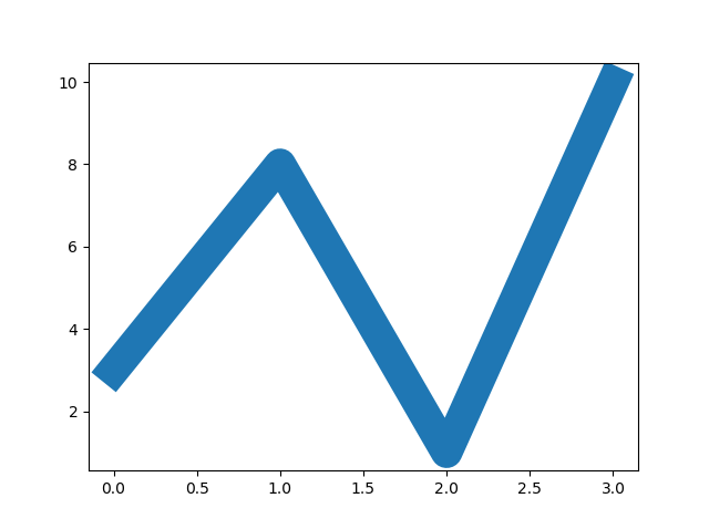
linewidth
设置线的宽度,fmt里面好像没有这个
缩写成lw
ypoints = np.array([3, 8, 1, 10])
plt.plot(ypoints, linewidth = '20.5')
plt.show()
绘制多条线
你可以通过简单地添加更多的plot .plot()函数来绘制任意多的线
y1 = np.array([3, 8, 1, 10])
y2 = np.array([6, 2, 7, 11])
plt.plot(y1)
plt.plot(y2)
plt.show()

还可以通过在相同的plt.plot()函数中为每条直线添加x轴和y轴的点来绘制多条直线
y1 = np.array([3, 8, 1, 10])
y2 = np.array([6, 2, 7, 11])
plt.plot(y1)
plt.plot(y2)
plt.show()  # 我们只指定y轴上的点,这意味着x轴上的点得到默认值(0,1,2,3)
x和y值成对出现
x1 = np.array([0, 1, 2, 3])
y1 = np.array([3, 8, 1, 10])
x2 = np.array([0, 1, 2, 3])
y2 = np.array([6, 2, 7, 11])
plt.plot(x1, y1, x2, y2)
plt.show()
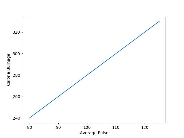
标签和标题
xlabel()和ylabel()
x = np.array([80, 85, 90, 95, 100, 105, 110, 115, 120, 125])
y = np.array([240, 250, 260, 270, 280, 290, 300, 310, 320, 330])
plt.plot(x, y)
plt.xlabel("Average Pulse")
plt.ylabel("Calorie Burnage")
plt.show()
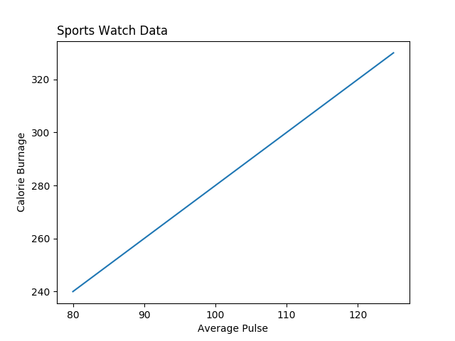
title()
标题,写在最上面
x = np.array([80, 85, 90, 95, 100, 105, 110, 115, 120, 125])
y = np.array([240, 250, 260, 270, 280, 290, 300, 310, 320, 330])
plt.plot(x, y)
plt.title("Sports Watch Data")
plt.xlabel("Average Pulse")
plt.ylabel("Calorie Burnage")
plt.show()

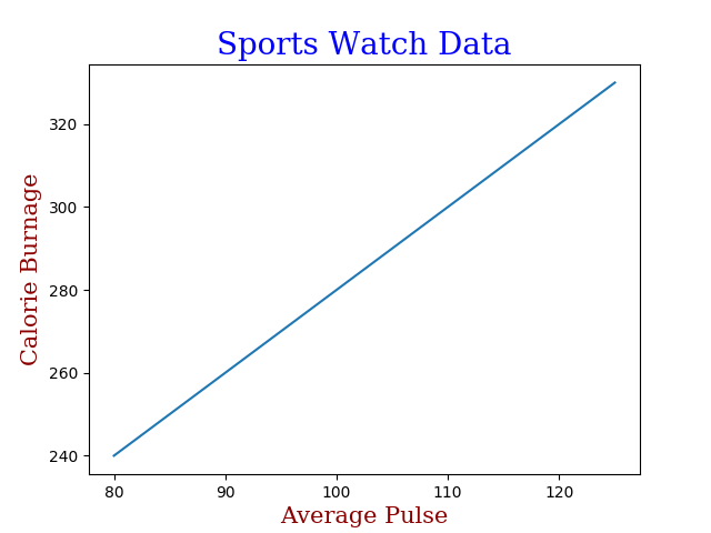
参数fontdict 给标题和标签设置样式
这个fontdict拿到的实参格式,就是css格式
x = np.array([80, 85, 90, 95, 100, 105, 110, 115, 120, 125])
y = np.array([240, 250, 260, 270, 280, 290, 300, 310, 320, 330])
font1 = {'family':'serif','color':'blue','size':20}
font2 = {'family':'serif','color':'darkred','size':15}
plt.title("Sports Watch Data", fontdict = font1)
plt.xlabel("Average Pulse", fontdict = font2)
plt.ylabel("Calorie Burnage", fontdict = font2)
plt.plot(x, y)
plt.show()
loc参数确定title的位置
可选:left、right、center(默认)
x = np.array([80, 85, 90, 95, 100, 105, 110, 115, 120, 125])
y = np.array([240, 250, 260, 270, 280, 290, 300, 310, 320, 330])
plt.title("Sports Watch Data", loc = 'left')
plt.xlabel("Average Pulse")
plt.ylabel("Calorie Burnage")
plt.plot(x, y)
plt.show()
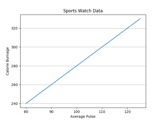
网格线
plt.grid()方法添加网格线
x = np.array([80, 85, 90, 95, 100, 105, 110, 115, 120, 125])
y = np.array([240, 250, 260, 270, 280, 290, 300, 310, 320, 330])
plt.title("Sports Watch Data")
plt.xlabel("Average Pulse")
plt.ylabel("Calorie Burnage")
plt.plot(x, y)
plt.grid()
plt.show()

指定要显示的网格线的轴向
grid()里面的参数axis表示显示的是x轴还是y轴还是都显示 x、y、both
x = np.array([80, 85, 90, 95, 100, 105, 110, 115, 120, 125])
y = np.array([240, 250, 260, 270, 280, 290, 300, 310, 320, 330])
plt.title("Sports Watch Data")
plt.xlabel("Average Pulse")
plt.ylabel("Calorie Burnage")
plt.plot(x, y)
plt.grid(axis = 'x')
plt.show()

plt.grid(axis = 'y')
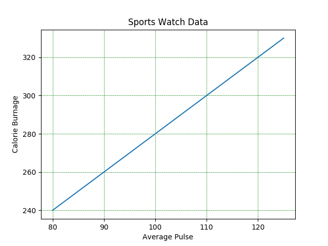
给网格线设置样式
你也可以设置网格的线条属性,像这样:grid(color = ‘color’, linestyle = ‘linestyle’, linewidth = number)
x = np.array([80, 85, 90, 95, 100, 105, 110, 115, 120, 125])
y = np.array([240, 250, 260, 270, 280, 290, 300, 310, 320, 330])
plt.title("Sports Watch Data")
plt.xlabel("Average Pulse")
plt.ylabel("Calorie Burnage")
plt.plot(x, y)
plt.grid(color = 'green', linestyle = '--', linewidth = 0.5)
plt.show()
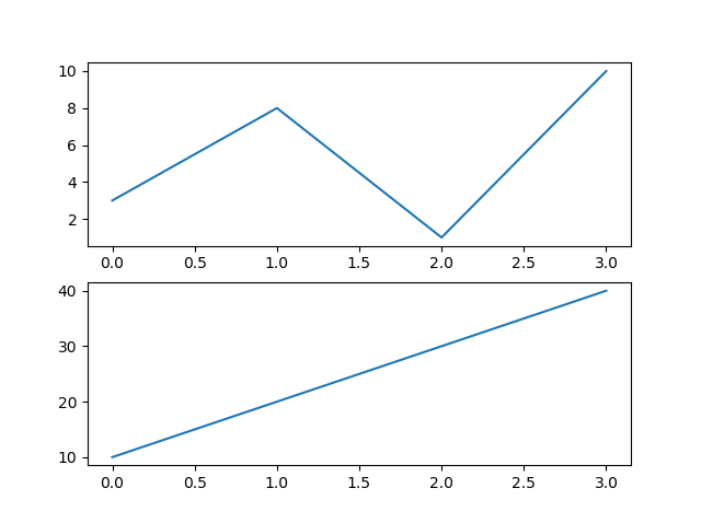
子图
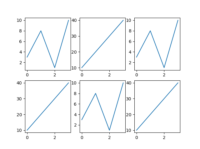
subplot()放多张图
plt.subplot(a, b, c) 这个视图被分成了a行b列,均匀切割,并且切换当前这个图到第c个图(一共a*b个)
#plot 1:
x = np.array([0, 1, 2, 3])
y = np.array([3, 8, 1, 10])
plt.subplot(2, 1, 1)
plt.plot(x,y)
#plot 2:
x = np.array([0, 1, 2, 3])
y = np.array([10, 20, 30, 40])
plt.subplot(2, 1, 2)
plt.plot(x,y)
plt.show()
x = np.array([0, 1, 2, 3])
y = np.array([3, 8, 1, 10])
plt.subplot(2, 3, 1)
plt.plot(x,y)
x = np.array([0, 1, 2, 3])
y = np.array([10, 20, 30, 40])
plt.subplot(2, 3, 2)
plt.plot(x,y)
x = np.array([0, 1, 2, 3])
y = np.array([3, 8, 1, 10])
plt.subplot(2, 3, 3)
plt.plot(x,y)
x = np.array([0, 1, 2, 3])
y = np.array([10, 20, 30, 40])
plt.subplot(2, 3, 4)
plt.plot(x,y)
x = np.array([0, 1, 2, 3])
y = np.array([3, 8, 1, 10])
plt.subplot(2, 3, 5)
plt.plot(x,y)
x = np.array([0, 1, 2, 3])
y = np.array([10, 20, 30, 40])
plt.subplot(2, 3, 6)
plt.plot(x,y)
plt.show()
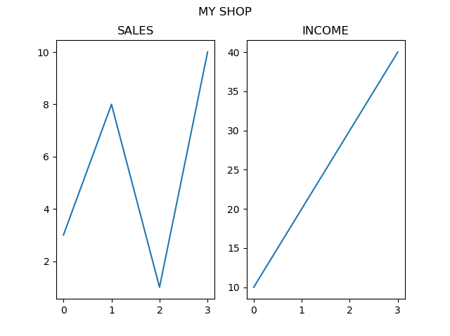
标题
tips:每个子图都可以加标题
#plot 1:
x = np.array([0, 1, 2, 3])
y = np.array([3, 8, 1, 10])
plt.subplot(1, 2, 1)
plt.plot(x,y)
plt.title("SALES")
#plot 2:
x = np.array([0, 1, 2, 3])
y = np.array([10, 20, 30, 40])
plt.subplot(1, 2, 2)
plt.plot(x,y)
plt.title("INCOME")
plt.show()
如果用了subplot的话,总的图还可以用suptitle()来添加一个大标题
#plot 1:
x = np.array([0, 1, 2, 3])
y = np.array([3, 8, 1, 10])
plt.subplot(1, 2, 1)
plt.plot(x,y)
plt.title("SALES")
#plot 2:
x = np.array([0, 1, 2, 3])
y = np.array([10, 20, 30, 40])
plt.subplot(1, 2, 2)
plt.plot(x,y)
plt.title("INCOME")
plt.show()
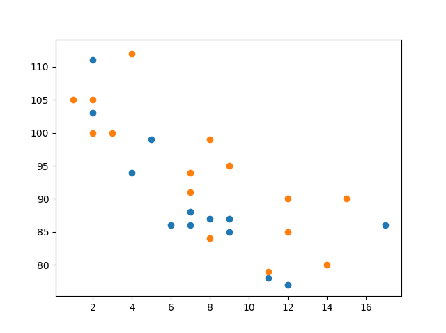
散点图
用scatter()创造一个散点图
#day one, the age and speed of 13 cars:
x = np.array([5,7,8,7,2,17,2,9,4,11,12,9,6])
y = np.array([99,86,87,88,111,86,103,87,94,78,77,85,86])
plt.scatter(x, y)
#day two, the age and speed of 15 cars:
x = np.array([2,2,8,1,15,8,12,9,7,3,11,4,7,14,12])
y = np.array([100,105,84,105,90,99,90,95,94,100,79,112,91,80,85])
plt.scatter(x, y)
plt.show()
操作基本上和plot是一样的,实际上我感觉plot把那个线的参数设置成空,然后把点的参数设置成o,就等于这个散点图了
color参数(缩写c)
基本上类似
plt.scatter(x, y, color = 'hotpink')
plt.scatter(x, y, color = '#88c999')
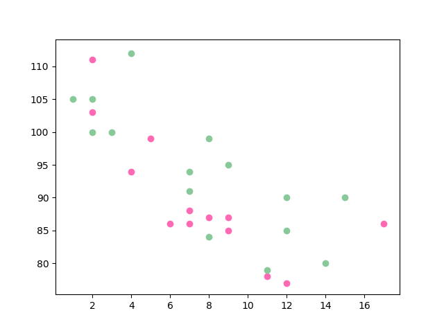
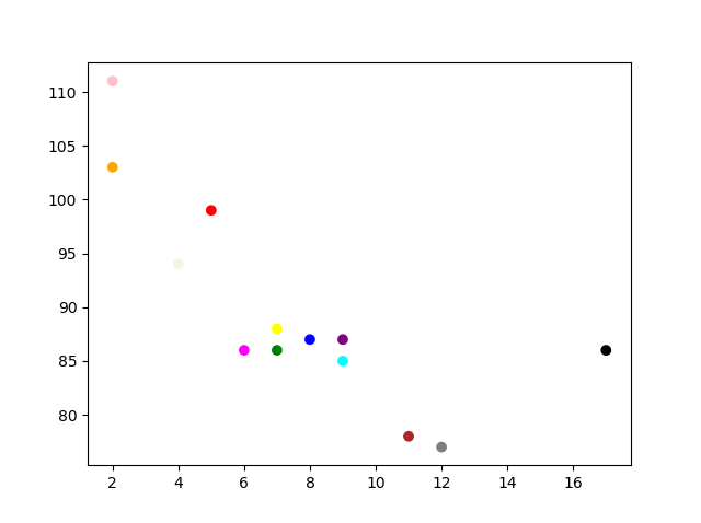
你甚至可以通过使用一个颜色数组作为c参数的值来为每个点设置特定的颜色
x = np.array([5,7,8,7,2,17,2,9,4,11,12,9,6])
y = np.array([99,86,87,88,111,86,103,87,94,78,77,85,86])
colors = np.array(["red","green","blue","yellow","pink","black","orange","purple","beige","brown","gray","cyan","magenta"])
plt.scatter(x, y, c=colors)
plt.show()
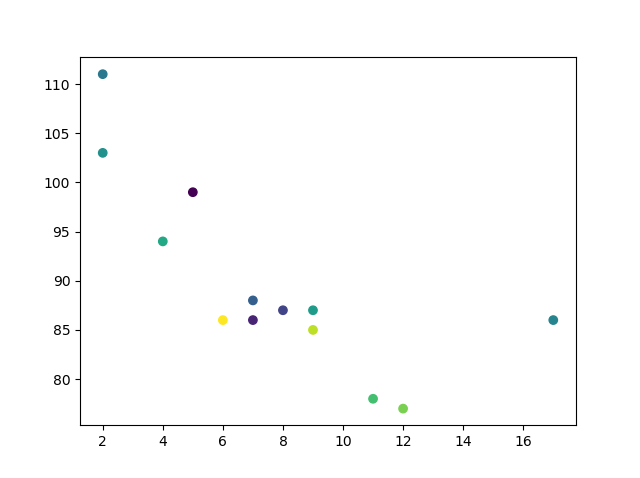
colirmap
Matplotlib模块有许多可用的色彩图。
colormap就像一个颜色列表,其中每个颜色都有一个从0到100的值。
下面是一个色彩图的例子:

这个配色图被称为“viridis”,如你所见,它的范围从0(紫色)到100(黄色)
你可以用关键字参数cmap和colormap的值来指定色彩图,在本例中是’viridis’,它是Matplotlib中可用的内置色彩图之一。
另外,你必须创建一个包含值的数组(从0到100),每个点对应一个散点图中的值
x = np.array([5,7,8,7,2,17,2,9,4,11,12,9,6])
y = np.array([99,86,87,88,111,86,103,87,94,78,77,85,86])
colors = np.array([0, 10, 20, 30, 40, 45, 50, 55, 60, 70, 80, 90, 100])
plt.scatter(x, y, c=colors, cmap='viridis')
plt.show()
你可以在绘图中使用plt.colorbar()语句
plt.colorbar()
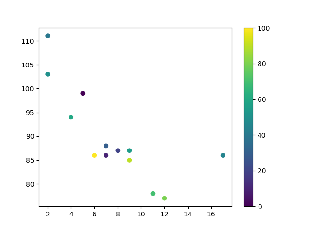
我感觉使用色彩图应该就是要和这个colorbar一起用才有意义,不然我也可以通过给每个点指定颜色来实现colormap(复杂一点点)(内置的色彩图有点多,这里不放了,自己查看看吧)
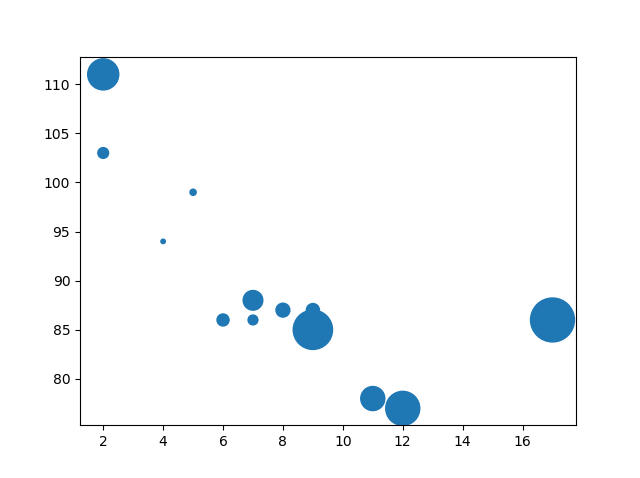
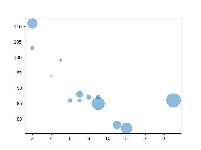
大小
参数s来修改大小
sizes = np.array([20,50,100,200,500,1000,60,90,10,300,600,800,75])
plt.scatter(x, y, s=sizes)
和c一样,都可以整花活,给每一个点都整个不同的大小
透明度
参数alpha指定透明度 0~1
plt.scatter(x, y, s=sizes, alpha=0.5)
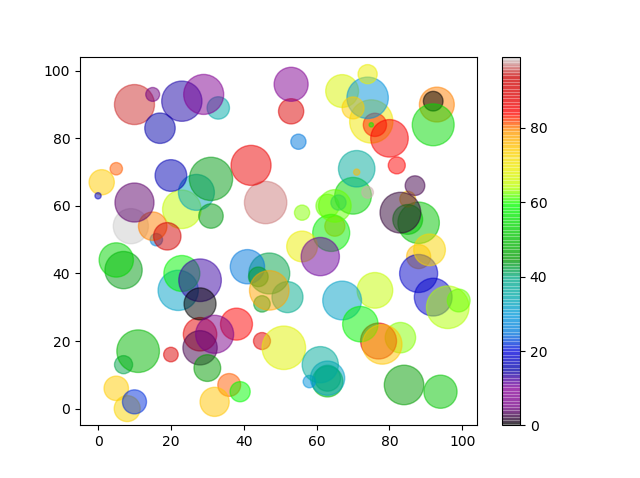
整个花活儿
x = np.random.randint(100, size=(100))
y = np.random.randint(100, size=(100))
colors = np.random.randint(100, size=(100))
sizes = 10 * np.random.randint(100, size=(100))
plt.scatter(x, y, c=colors, s=sizes, alpha=0.5, cmap='nipy_spectral')
plt.colorbar()
plt.show()